After about 8 hours of programming, I got mitosis and stem cell differentiation working in the genetic engine yesterday. Pictured is a 1840 neuron columnar nucleus, grown in a linear fashion initially, then radiating outward via differentiating mitosis. SynthNet is now able to regulate growth (so it isn’t cancerous), as well as direct growth based on protein signaling markers, allowing it to grow differentiated structures.

The last few months I’ve been building out SynthNet’s genetic engine. Each neural structure runs a genetic virtual machine within it that executes genetic instructions obtained from its virtual DNA. Additionally, to make the job of creating this DNA easier, I’ve written a genetic assembly language and a compiler that transforms genetic programs into virtual DNA. The genetic instruction set supports reading and writing any attribute of a structure, including its morphology, ion and protein synthesis, changes in membrane capacitance, growing channels and receptors, changing permeabilities, causing mitosis (soon) or apoptosis, etc. All in all there are around 100 genetic instructions.

The first picture below is a dendritic arbor I grew using a single strand of virtual DNA . I don’t have enough termination functionality to prevent cancerous growth at this point (soon), but I do have enough to control process growth origination and angle. This was grown with 3 codons worth of DNA – almost nothing. Below that was a snowflake formation, also using 3 codons worth of DNA.

Fixed the rendering so it processed diameter properly, then added in a color graph to show corresponding color to potential, and a real time graph to plot the membrane potential of a specified neuronal process. This will definitely make monitoring and debugging a lot easier

I’ve been working on the rendering engine for SynthNet, so both the neuronal morphologies can be seen, and membrane potential and other activity can be visualized through color coding, like in an fMRI.

This is an example of it in action so far. The models look pretty clunky and simple, but that’s by design – I just want a simple, lightweight viewer that doesn’t take up too much CPU time. This example shows two neurons and a synapse – one with 3 dendrites and an axon, with a synaptic gap between the post-synaptic neuron, consisting of only a small neuronal segment (a dendrite). Membrane potential is shaded in red, with white representing -70mV, and bright red representing 30mV.

The top picture shows the two neurons at rest. In the second picture, I inject current into one of the dendrites, and you can see the current flowing up its process into neighboring dendrites and the soma, getting weaker as it goes due to attenuation.

In the final picture, we see a large amount of current injection into all dendrites, causing an action potential and release of neurotransmitters into the synaptic gap, which causes an influx of ions in the post-synaptic neuron, depolarizing the membrane potential, as can be see with the post-synaptic neuron also showing red shading.

When I first got the code working and watched all this happening live, it was definitely one of those wow moments.

I finished up the code that handles the number of neurotransmitter vesicles that fuse with the plasma membrane (and release into the synapse) in relation to calcium concentration in terminals. The code will autoselect the appropriate method of computation depending on the probability and total number of vesicles. For a large number of vesicles and low probability, the Poisson model is used. For a large number of vesicles and high probability, the binomial estimation method is used. For a low number of vesicles, the full binomial method is used.

Love the Poisson graph, as it has enough vesicles to get a good curve, but low enough probability to show the stochastic nature of the process.

Synthnet’s very first synaptic transmission tonight! Pictured are the membrane potentials of two neurons sharing a synapse.

You can see the action potential travel down the axon of the presynaptic neuron, which causes a calcium influx in the axonal boutons, which then releases glutamate vesicles into the synaptic cleft. Ligand gated glutamate channels in the postsynaptic neuron cause sodium channels to open, which causes an action potential in the post synaptic neuron, and travels down its axon, as shown.

In the next post, I’ll be outlining the methods used to calculate the vesicle release rate.

Pictured here are the membrane potential graphs from a complete virtual neuron from SynthNet. This neuron was comprised of 3 dendritic structures of smaller diameter, a larger soma, and a hillock and long axon.

On the drawing, I labeled what point on the representation neuron each graph pertains to. You can see me feeding high frequency, medium frequency, and low frequency oscillating voltage into the dendritic arbor at different points, and then you can see them temporally and spatially summating at the axon hillock until they hit -40mV, which then triggers an action potential down the axon, which propagates from segment to segment all the way down (See the three spikes very close to each other – thats the pulse moving down the axon). I keep the oscillation up and trigger 2 more action potentials too after the refractory period is over. You can also see the backpropagation of voltage go back through the soma into the dendrites where retrograde messengers will be released (see the jump back on the dendrites around time 500, in relation to getting electrotonic current from the axons).

This demonstrates the proper interaction between electrotonic potential, membrane potential, and ionic current flow.

Continuing on posting some past work to get the blog up to date, here are some graphs showing completion of the Hodgkin Huxley method of processing voltage gated ion channels. At this point, the neural network supports adding ion channels to the plasma membrane with different gating types, including voltage gates as well as voltage gates with inactivation gates (as well as ion pumps, though these are not processed by HH).

Akin to how protein subunit types give rise of the type of channel and gates of a physical ion channel, attributes associated with a SynthNet ion channel control what kind of channel and gates it possesses. Additional properties such as membrane threshold potential, permeability, and refractory period control the behavior of the voltage gated ion channels.

Below are some graphs with a two connected neural processes, the latter containing voltage gated sodium channels (with inactivation gates) and voltage gated potassium channels, constructed to behave as normal neural structures do during the action potential process. The first structure (membrane potential shown in blue) was clamped at -30mV for different periods of time in each graph. Shown is red is the membrane potential of the second structure. The left graphs show regular firing with different refractory periods, while the right graphs show burst and oscillating potentials (caused by the rate and magnitude of repolarization remaining higher than the threshold potential, coupled with a very short refractory period).

In the next post, I’ll be showing the interaction of action potential (via HH) and electrotonic potential (via cable and capacitance calculations) over a more complex morphology.

Though I haven’t updated the blog in a while, I’ve really been going full-steam on the neural emulator. I’ve been taking screenshots as I go, so over the next day or so I’m going to try to make a few posts with those shots to get everything up to speed on the blog. Also, thanks for all the comments on other posts! I’ll be getting back to them soon (this weekend).

The first big update concerns processing electrotonic potential across the cell and the plasma membrane. In my previous post, I talked a bit about using the cable equation for distribution of current. As of now, I still make use of the cable equation for distributing potential across the cell. This takes into account the length and circumference of the segment in question, in addition to internal resistance, and resistance across the plasma membrane. Also, in order to appropriately address membrane moieties, calculations will also take into account the capacitance of the membrane. This allows not only a more realistic build-up of potential to occur to allow things like temporal summation to work properly, but also allow us to emulate myelination, in which electrotonic potential is subjected to a change in attenuation due to higher resistance and lower capacitance of the plasma membrane.

Below is a membrane potential graph generated from a simple structure consisting of 3 segments. The first segment is clamped with oscillating voltage, with structure 2 connected to 1, and 3 to 2. We can see the subsequent structures increase and decrease according to their distance from structure 1. The curve is controlled by the capacitance and resistance of the plasma membrane:

Note that membrane resistance is calculated via ionic permeability. This is a simple graph and the following posts will show some more interesting graphs with the effects of spatial summation and changes in resistance illustrated, but this one is very clear at showing the expected curve associated with a capacitor.

Next post illustrates the completion of Hodgekin-Huxley calculations for voltage-gated ion channels.

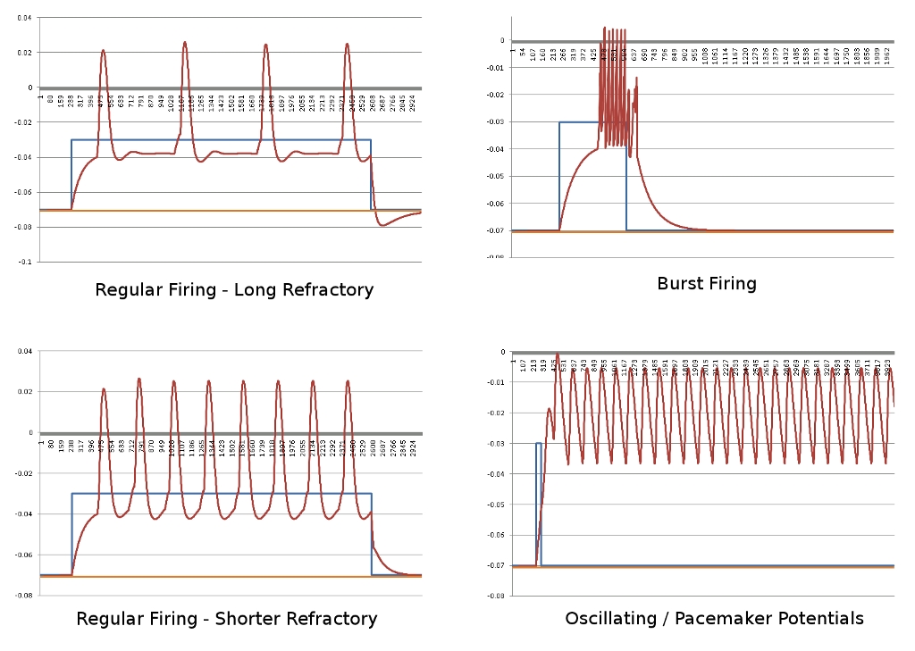
Progress marches forward on the Neural Emulator front. I’ve currently fleshed out the functionality as described by the cable equation, that describes how voltage/current flows down neural structures. This will allow adjacent sections of the cellular membrane to propagate changes in potential, thereby properly emulating the action potential. Before I can advance at all, I need to ensure that the action potential sequence models properly, since this is such core functionality.

Voltage Propagation

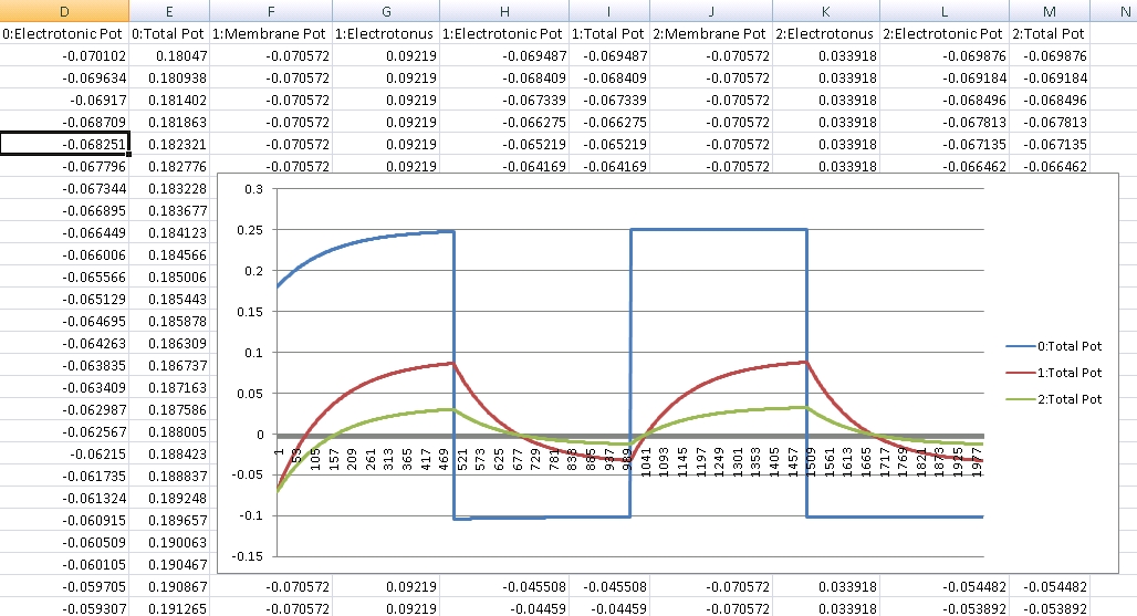
In the following graph, I’ve setup a neuron consisting of 4 structures. For the purposes of this test, it doesn’t really matter what the structures themselves are, but you could think of it as 4 sections of a fiber in a dendritic arbor. They all start out with the same intra and extracellular ionic concentrations, membrane permeability, and size. They are arranged linearly, where structure 0 is connected to 1, which is connected to 2, which is connected to 3. In this experiment, I increased in the extracellular concentration of Sodium surrounding structure 0. The graph shows both the local potential (potential for the cell membrane when isolated from adjacent membranes), as well as the total potential (when accounting for adjacent membranes).

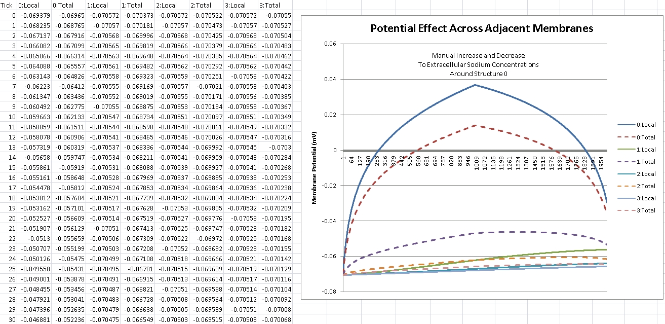
As can be seen, as we increase the extracellular Sodium concentration, the cell membrane of structure 0 depolarizes as the local potential goes positive. Though the Sodium concentration surrounding the adjacent structures has (mostly) not changed, as can be seen by their local potentials, their total potential increases accordingly due to their proximity to structure 0. The closer they are (structure 1 is the closest), the more their membrane potential is affected. The effects of such are calculated by voltage difference, connecting membrane area, and distance between them. So this test came out successful.

Hodgekin-Huxley

In addition, I’m about half way finished with integrating the Hodgekin-Huxley model and associated equations in with calculating the permeability of gated ion channels, specifically for voltage and inactivation gates. This will ensure that the ion permeability adjusts correctly depending on the membrane potential. However, before I was able to move forward on HH, I needed to ensure membrane potentials were propagating properly, which is why the work above was important. More on this soon!